Predicting spatial gene expression from tissue images

Spatial transcriptomics measures which genes are active at each location in a tissue section, but it is expensive and uses up the section. H&E staining is cheap and sits on almost every clinical slide. If morphology carries enough information, a model trained on paired H&E and spatial RNA could estimate expression maps for new tissue and point to regions worth measuring. A prediction is a hypothesis about the tissue, not a new measurement, so the real question is narrower: in a patient the model has never seen, how much of the spatial RNA pattern can be read from the image, and which way of training gets closest?

The data are three colorectal cancer patients profiled with Visium HD and analyzed at 8 µm bins. A bin is a grid square, not a cell. Most measured counts are zero, and a zero can reflect sparse sampling as easily as true absence.

Every model uses the same frozen image features from an existing pathology encoder (HIPT) and the same small neural network. What changes is the training recipe. MSE fits log-transformed counts with squared error. NB fits raw counts with a negative binomial likelihood, the standard model for overdispersed count data. ZINB adds an explicit probability of extra zeros. Each recipe also changes the training target and how a prediction is read out, so this compares recipes, not loss functions in isolation.

The test is at the patient level: train on two patients, evaluate on the third, and rotate so each patient is held out once. Gene selection (about 3,000 variable genes plus a fixed list of 94 markers), feature normalization, learning-rate choice and checkpoint choice use only the training patients. The held-out patient's RNA is touched only at final evaluation. Each method gets its own tuned learning rate and five fresh training seeds, so no recipe is judged at another recipe's settings. I designed and ran these experiments, built the GPU pipelines, and presented the results, with guidance from PI Tianlong Chen and mentors Mufan Qiu and Ruichen Zhang, and in collaboration with Yi Zhang (Duke University).

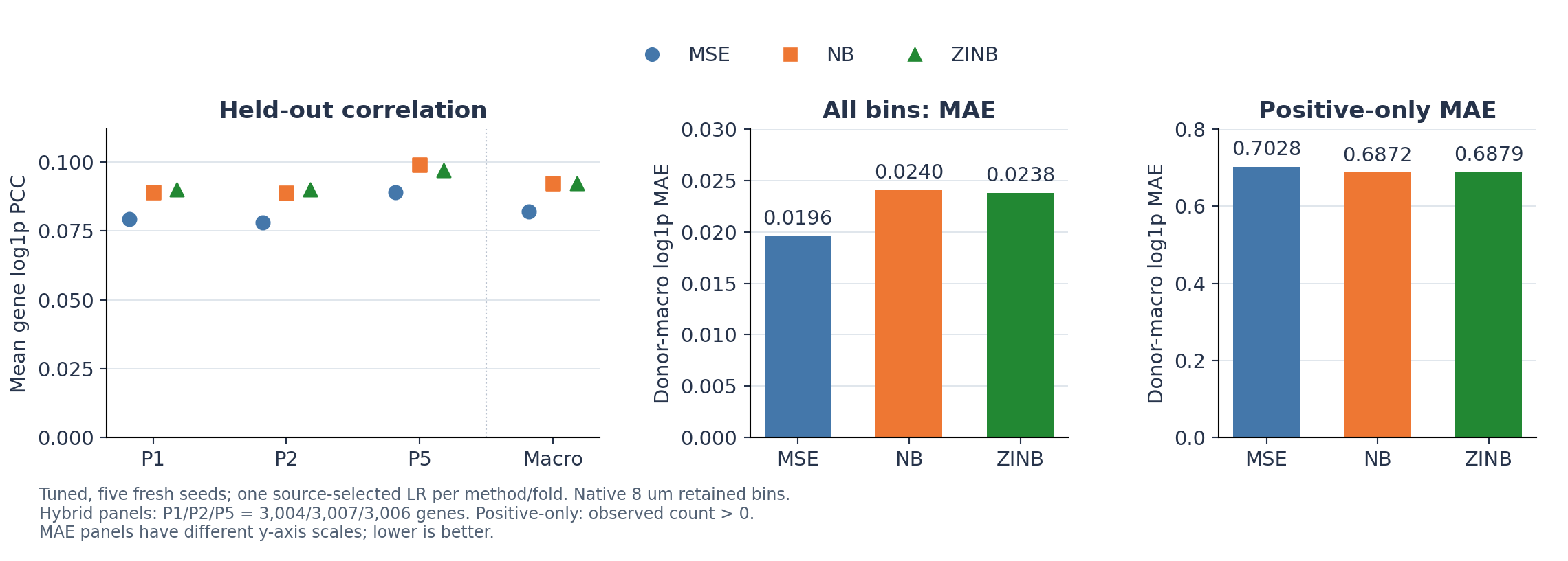
In all three held-out patients, both count models tracked a gene's spatial highs and lows better than MSE. They also made larger errors averaged over every bin. Those two facts do not conflict. Correlation asks whether a predicted map rises and falls where the measured one does; absolute error asks how far off each bin's value is. When most counts are zero, predicting close to zero everywhere can score low error while saying little about where a gene is. The count models spread predicted signal into more bins: correlation rose, error at measured-positive bins fell, and error across all bins rose. ZINB gave no consistent advantage over plain NB.

The correlations are low in absolute terms because the panel includes thousands of genes that are barely visible in morphology. The result is the comparison between recipes, not the level. Three patients cannot establish performance on a wider population.

The lesson I take most from this project is about evaluation. An early result seemed to show a large advantage for one training objective, but the models had been trained at different learning rates; once settings were matched, the gap shrank a lot. A more complex generative approach (flow matching) also gave no stable gain in controlled runs. Since then, every comparison is matched before it is interpreted.

The biggest gap is biological. Brighter, smoother maps are not evidence that a model found real cells. In some regions the count models predict broad signal where few counts were measured, and that needs an independent reference to judge. The next step is to score predictions against independently annotated tissue regions, which has not been done yet. Proposed follow-ups, none of them run yet, would test where the remaining limits come from: newer image encoders, simple spatial-neighborhood context, and a model that builds expression from predicted cell-type mixtures.